Building a Neural Network to Recognize Handwritten Digits
In this project I built a neural network entirely from scratch in MATLAB to classify handwritten digits from the MNIST dataset. With no toolboxes and full manual control over architecture, activation, and optimization, this was a hands-on crash course in how neural networks really work — and how to make them work well.
🧠 Network Architecture
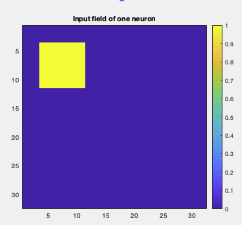
The network has four layers, including two 28×28 “map” layers with field-fraction 0.25, meaning each neuron connects only to a local region of the previous layer. This reflects the idea that nearby pixels influence each other more than distant ones — similar to receptive fields in the visual system.
Layer Structure
- Input: 28×28 grayscale image (784 features)
- Layer 2: 28×28 map layer, locally connected
- Layer 3: 28×28 map layer, locally connected
- Layer 4 (Output): 10 neurons — one for each digit 0–9
Dense Projection: Both Layer 2 and Layer 3 connect directly to the output layer, so the final weights form a 10×1568 matrix: \[ W^{(4)} = \text{weights from } [y^{(2)}; y^{(3)}] \rightarrow y^{(4)} \]
⚙️ How It Works: Forward Propagation
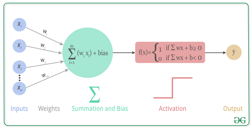
Step 1: Weighted Sum
Each neuron receives input from the previous layer via weights: \[ v_i^{(l)} = \sum_j W_{ij}^{(l)} y_j^{(l-1)} + b_i^{(l)} \]
Step 2: Activation
The signal passes through an activation function — here, a custom one called relog: \[ y_i^{(l)} = \max\left(0, \text{sgn}(v_i^{(l)}) \cdot \log(1 + |v_i^{(l)}|)\right) \] This activation smooths small gradients while preserving nonlinearity, helping the network learn complex patterns.
Step 3: Output & Softmax
The final output layer is affine, followed by softmax to convert raw scores into probabilities: \[ y_i = \frac{\exp(y^{(4)}_i)}{\sum_j \exp(y^{(4)}_j)} \]
🎯 Training the Network
Step 1: Loss Function
We use one-hot labels and calculate the error as: \[ \mathbf{e} = \mathbf{y} - \mathbf{y}^*, \quad L = \frac{1}{2} \mathbf{e}^\top \mathbf{e} \]
Step 2: Backpropagation
To adjust the weights and biases, we compute the gradients of the loss using the chain rule, propagating error backwards layer-by-layer.
The final gradient for the output layer is computed explicitly outside the main function: \[ \frac{\partial L}{\partial v^{(4)}} = \mathbf{y} - \mathbf{y}^* \]
🧮 Optimization: Adam Algorithm
To update the weights, we use the Adam optimizer, which improves standard stochastic gradient descent (SGD) by using adaptive learning rates and momentum:
- Maintain moving averages of gradients (mean and squared)
- Update each parameter:
- Learning rate: ( η = 0.001 )
- Includes bias correction for moment estimates
Adam is fast and stable — ideal for noisy updates and sparse data.
🧪 Results
After 10 training epochs (60,000 examples, in minibatches of 100), the network achieved:
98.5% accuracy on the MNIST test set
(Only ~150 errors out of 10,000 images)
I would like to thank Dr. Douglas Tweed who created this project for the course PSL432: Theoretical Physiology .